Article information

Korean J Otorhinolaryngol-Head Neck Surg. 2023;66(7):447-454

Publication date (electronic) : 2023 May 30

doi : https://doi.org/10.3342/kjorl-hns.2021.00780

Seung Cheol Han, Hae Chan Park, Ye Jin Byun, Myung-Whan Suh, Jun Ho Lee, Seung-Ha Oh, Moo Kyun Park

Department of Otorhinolaryngology-Head and Neck Surgery, Seoul National University Hospital, Seoul National University College of Medicine, Seoul, Korea

한승철, 박해찬, 변예진, 서명환, 이준호, 오승하, 박무균

서울대학교 의과대학 서울대학교병원 이비인후과학교실

Address for correspondence Moo Kyun Park, MD, PhD Department of Otorhinolaryngology-Head and Neck Surgery, Seoul National University Hospital, Seoul National University College of Medicine, 101 Daehak-ro, Jongno-gu, Seoul 03080, Korea Tel +82-2-2072-2446 Fax +82-2-745-2387 E-mail aseptic@snu.ac.kr

Received 2021 August 9; Revised 2022 December 23; Accepted 2022 December 26.

Trans Abstract

서 론

중이는 외이도와 내이의 사이에 위치하고 있으며, 외이도에서 수집된 소리 신호를 진동으로 변경하여 내이로 전달한다. 이러한 전달을 위하여 중이는 외이도와 내이 사이의 임피던스를 맞추는 기능을 하고 있다. 중이의 기능에 방해가 되는 것은 중이강 안의 저류액이나 염증, 진주종, 이소골 연결성의 이상 등으로, 이들의 원인으로 청력의 전달에 문제가 생기면 순음청력역치검사나 고막운동도검사(tympanometry)를 통해 그 원인을 추측해보게 된다 [1-3].

기존의 tympanometry 검사는 대개 226 Hz와 같은 한 주파수에서의 어드미턴스(임피던스의 역수, admittance) 측정한다. 이를 통해 중이의 경직성(stiffness)과 임피던스를 반영하고, 이러한 결과를 통해 중이의 질환에 대한 예측을 한다. 그러나 이렇게 한 주파수에 특징적인 정보는 충분한 정보라고 할 수 없으며, 그렇기 때문에 기존의 tympanometry는 여러 제한점들이 있다. 그 중에서도 중이의 삼출액(fluid)은 없으나 이관의 기능이상으로 음압이 발생하는 C형(type C) 결과의 경우 실제 임상적인 검진 시 그러한 원인보다도 중이의 fluid가 있는 경우가 원인이 되기도 한다[4]. 또한, 이경화증의 경우, tympanometry를 시행하였을 때 대부분의 경우의 결과는 정상과 큰 차이를 보이지 않는 경우가 많다[5].

광대역 고막 흡수도 검사(wideband tympanometry, WBT)는 이러한 기존의 tympanometry의 단점들을 극복하고자 사용되기 시작하였다[6,7]. WBT는 기존의 tympanometry와는 달리 흡수도(absorbance)라는 값을 사용하고 있으며, 중이로 들어가 흡수되는 소리에너지와 외이로 넓은 주파수범위에서 반사되어 나오는 정도를 측정하여 기존에 226 Hz에서만 시행하던 tympanometry의 단점을 극복하였다[8-11]. 이와 함께 추가적으로 공명주파수(resonance frequency)나 고점에서의 압력(peak pressure) 등의 값도 얻을 수 있다[12].

WBT에 관한 연구들로는 이소골들과 관련한 연구들이 많았다. 이경화증의 경우 정상에 비해 250-2000 Hz에서 평균 absorbance 수치가 낮고, receiver operating characteristic (ROC) curve를 이용한 분석상 250-1500 Hz 사이의 WBT의 absorbance 값을 사용하여 이경화증을 유의하게 진단할 수 있고, 정상군과 구분할 수 있다고 보고된 바 있다[13]. 또한, 이경화증이 진행됨에 따라 resonance frequency 값이 증가한다는 보고도 있었고[10,11], 시체를 이용한 연구에서는 등골의 고정(stapes fixation)이 있는 경우 2000 Hz를 넘는 주파수에서는 반사도(reflectance)가 감소한다고 보고된 바도 있었다[14].

본 연구진 또한 이전에 2019년 연구에서 전음성 난청 환자들에서의 WBT 결과를 비교하여 전음성 난청질환을 구분한 바 있다. 당시에는 전음성 난청 환자들에서의 WBT 결과를 고막천공, 이소골 문제, 유양동의 문제로 구분하여 비교하였었다[15]. 당시 연구 결과로는 이소골 문제가 있는 전음성 난청 환자들의 경우 peak pressure가 낮았다는 점과 고주파수에서의 absorbance가 떨어진다는 점이 있었다. 또한 유양동의 문제가 있는 전음성 난청 환자들의 경우는 모든 주파수에서 absorbance가 떨어진다는 결과를 얻은 바 있다.

기계학습(machine learning)이란, 특정 데이터를 통해서 예측 함수를 만들어 내는 과정이다. 특히나 다양한 소스의 데이터를 이용하여 정확한 예측을 해내는 함수를 만들어 내는 데에 상당히 유용한 것으로 알려져 있다[16-18].

본 연구에서는 정상(normal), 만성중이염(chronic otitis media, COM), 이경화증(otosclerosis), 이관개방증(patulous eustachian-tube disorder, ETD)으로 진단된 환자들에서 주파수별 absorbance 데이터와 resonance frequency, peak pressure 등의 데이터를 machine learning을 통해 분석하여 상기 진단명들에 대한 WBT의 진단적 특징에 대해 알아보고자 하였다.

대상 및 방법

본 연구에서는 2015년 1월부터 2021년 2월까지 서울대학교병원 이비인후과 외래에 내원하여 WBT 검사를 시행한 165명의 환자들을 대상으로 좌우 귀에 대해 각각 분석하였다. 이들의 외래기록, 수술기록, 입원기록 등을 포함한 의무기록 자료를 이용하여 후향적 분석을 시행하였고, 연구에서 정상의 진단은 이과 진료 10년 이상의 전문의들이 내린 진단이며 중이 질환은 임상양상, 고막소견, 청력검사 및 측두골 컴퓨터단층촬영검사(temporal bone computed tomography, TBCT) 소견을 통해 진단되었다. 본 연구는 서울대학교병원의 인증된 연구윤리 심의위원회(Institutional Review Board, IRB)의 승인을 받았다(IRB No. H-2103-046-1203).

WBT 검사를 시행한 귀들은 총 179개의 정상 귀들과 151개의 비정상 귀들로 구성되어 있었고, 비정상 귀들 중 만성중이염(COM)인 경우가 113개, 이경화증(otosclerosis)으로 진단된 경우가 14개, 이관개방증(ETD)으로 진단된 경우가 24개가 있었다. 만성중이염의 경우, 고막 천공이 있으면서 이루가 있는 경우를 모두 만성중이염으로 진단하여 연구에 포함시켰다. 이경화증의 경우 전음성 난청(Carhart’s notch)과 함께 TBCT상에서 fissula ante fenestrum이나 cochlea 주변의 방사성 투과성 병변이 있는 경우 혹은 환자 기록상 이경화증의 의심 하 등골절개술을 받은 경우로 진단하여 연구에 포함시켰다. 이관개방증의 경우, 환자의 자가강청 및 이충만감과 같은 임상증상과 함께 귀 내시경 검사상 호흡과 일치하는 고막의 내외측 움직임이 있거나, 임피던스 고막 운동성 계측(고막운동도, tympanometry)상에서 호흡을 멈춘 경우에는 A형의 정상적인 소견이나 코로 호흡을 빠르게 할 때는 고막운동도의 모양이 톱니 모양으로 변하는 경우를 이관개방증으로 진단하여 연구에 포함시켰다. 본 연구에서의 WBT 측정은 Titan System (ver. 3.4; Interacoustics Corp., Middelfart, Denmark)의 software package IMP440/WBT440 version v.3.2를 이용하여 진행하였다.

본 연구에서 WBT로 얻은 값으로는 peak pressure, resonance frequency, absorbance 데이터가 있었고, peak pressure, resonance frequency의 경우 Mann-Whitney test를 통하여 분석하였고, absorbance 데이터의 경우 peak pressure에서의 값들과 average pressure에서의 값으로 나누어 분석하였다. Absorbance 데이터의 경우 약 122개의 주파수(226-8000 Hz)에서의 absorbance를 측정하므로, 대상 수에 비해 변수의 수가 상당하다는 점을 고려하여, 본 연구에서는 machine learning 기법을 통계적으로 사용할 것을 결정하였다. 이에 peak pressure, resonance frequency 데이터와 absorbance 데이터, 환자들의 age 데이터를 함께 모델링(modeling)하여 machine learning 기법을 이용한 분석을 시행했다.

Machine learning에서는 학습집합(train set)의 결과값과 변수값을 많이 대입하여, 특정 변수값에 따른 결과값을 예측할 함수를 만들어 보고, 이러한 함수가 실제로 맞는지 검증(validation) 과정을 통해 확인하게 된다. Validation에 사용되는 검증집합(validation set)은 train set과는 다른 데이터를 사용해서 모델링이 제대로 되었는지 확인하게 된다. 마지막으로 테스트집합(test set)은 validation을 통해 사용할 예측 함수가 정해지고 난 후, 해당 함수의 예상되는 성능을 측정하기 위해 사용된다.

본 연구에서는 자료수가 많지 않아 자료를 train, validation, test set 3개로 나누지는 못했다. 본 연구의 각각의 Model들에서는 train set은 2015-2019년 자료로, test set은 2020-2021년 자료로 구성하였고, 별도의 validation set은 나누지 못했다. 본 연구에서 결과의 도출이 가능한 Model들은 3가지였고, Model 1의 경우 정상군과 만성중이염군의 비교, Model 2의 경우는 정상군과 이관개방증군의 비교, Model 3은 정상군과 만성중이염군, 이경화증군, 이관개방증군을 모두 합친 중이 질환군의 비교로 구성되었다(본 연구의 초기 목적과는 달리, machine learning 기법을 이용한 결과의 도출이 가능한 model들은 상기 3가지뿐이라, 본 연구에서는 상기 3가지 모델들에 대해서만 기술하게 되었다).

또한 본 연구에서 사용한 machine learning의 예측 함수는 기본적으로 로지스틱 회귀함수(logistic regression)로 설정되었는데, 최적화가 과도하게 진행되면 선형회귀계수(weight)의 크기도 과도하게 증가하게 된다. 그래서 이를 막기 위해 계수의 크기를 제한하는 제약조건을 가하며 모델링을 하는데, 그러한 모델링의 방식으로 least absolute shrinkage and selection operator (LASSO)와 elastic net이 있다[19]. LASSO와 elastic net은 변수선택법(variable selection)이 포함된 로지스틱 회귀함수이다[20,21]. LASSO와 elastic net 모두 결과변수와 관련성이 낮은 변수의 회귀계수를 0으로 추정(회귀계수 규제, regularization)하기 때문에, 변수선택(feature selection)과 모형구축이 같이 진행되는 것이다. 이러한 feature selection 결과로 LASSO, elastic net 방법으로 구한 최종 모형에는 관련성이 높은 일부 변수만이 포함되었다. LASSO에서의 hyperparameter lambda와 elastic net에서 lambda, alpha는 각각 10-fold cross-validation에서 area under the ROC (AUC)가 최대가 되는 값으로 선택하였다.

한편, 본 연구에서는 random forest 방식의 machine learning 기법도 추가로 시행하였는데, 이는 여러 decision tree (의사결정나무)를 합치는 방식이다. Decision tree란 나무가 뿌리와 잎으로 구성된 것처럼 변수값 하나하나를 기준으로 분류해 가는 machine learning 모형이다. Decision tree는 과적합 문제(overfit, 자료 수보다 변수의 수가 더 많아서 해당 자료에서는 예측을 잘 하지만, 새로운 다른 자료에서의 예측이 나쁨)가 있어서, 이를 보완하기 위해 여러 decision tree 예측 값을 합하여 예측하는 방식이 random forest인 것이다. 본 연구에서 random forest 후보 분리변수의 수(mtry)는 전체 feature 개수에서 1을 뺀 수의 제곱근(sqrt[변수개수-1])으로 사용하였으며, decision tree 개수(ntree)는 3000개를 사용하였다. Random forest는 앞의 방식들과 달리, 그 결과를 변수의 계수 값 형태로 제시하지 않고, 변수와 예측과의 중요도(importance)을 제시한다. Importance는 ‘accuracy’나 ‘Gini’라는 값을 통해 계산되고, 그 값이 클수록 중요도가 높다. Accuracy는 가령 데이터들을 1 또는 2로 분류하는 정확도이고, ‘mean accuracy decrease’는 특정 변수를 제외한 경우에 모형의 accuracy가 떨어지는 정도를 나타내며, 그렇기에 mean accuracy decrease 정도가 클수록 해당 변수의 중요도는 높아지게 된다. Gini는 decision tree가 얼마나 결과값을 잘 구분하였는지를 decision tree의 불순도(impurity)로 평가한다. Impurity는 예를 들어, 어떤 조건(age＞5, sex=F, X1≥50...)을 만족하는 경우에 Y=1로 예측을 하였으나, 그 조건에 해당하는 대상자에서 모두 Y=1인 경우에는 impurity가 0로 가장 낮고, 해당군에서 Y=1이 50%, Y=0이 50%인 경우에는 impurity가 가장 높다고 이해하면 된다. 이와 같이 각 변수가 impurity 감소에 기여하는지를 보는 것이 ‘mean Gini decrease’ 결과이다.

Machine learning 모델링을 위해 Rstudio를 주로 이용하였고, LASSO 및 elastic net 분석을 위해 ‘glmnet’ package를 사용하였다. 또한 random forest 분석을 위한 ‘randomForest’ package, AUC 분석을 위한 ‘pROC’ package도 사용하였다. 분석을 위한 주 software로는 SPSS software (ver. 21.0; IBM Corp., Armonk, NY, USA)와 Rstudio (ver. 4.0.3; RStudio Inc., Boston, MA, USA)를 사용하였다.

결 과

총 165명의 환자들의 좌우 귀, 330개의 귀를 대상으로 분석을 진행하였다. 연구에 참여한 대상들의 인구학적 특징은 유의미한 차이는 없었다(Table 1).

Table 1.

Patient demographics and wide tympanometry results

본 연구의 대상들에게 시행한 WBT에서 얻은 peak pressure와 resonance frequency 데이터들은 정규성을 띠지 않아, Kruskal-Wallis test를 통한 비모수 검정을 시행하였다. 이후 시행한 Mann-Whitney test를 통한 사후검정에서 정상군과 비교하였을 때, resonance frequency와 peak pressure 모두 만성중이염군에서만 유의미한 차이가 있었다(Table 1).

Fig. 1A은 모든 frequency에서의 WBT 자료를 평균화하여 pressure와 absorbance만을 나타낸 averaged tympanogram이다. 각각의 tympanogram들은 모두 0 daPa에서 고점을 보였고, 만성중이염군의 경우 flat한 형태를 보이는 것을 알 수 있다. 반면 이경화증군과 이관개방증군의 경우는 비교적 정상군에 비해 고점이 약간 낮아져 있고 음(-)의 daPa 구역에서는 정상군보다 absorbance가 증가됨을 알 수 있다.

Fig. 1.

Wideband tympanometry data of various middle ear disease. A: Averaged wideband tympanogram data. B: Averaged absorbance data at ambient pressure. C: Averaged absorbance data at peak pressure. COM, chronic otitis media; ETD, patulous eustachian-tube disorder.

Fig. 1B and C는 각기 ambient pressure와 peak pressure에서의 absorbance를 평균화하여 주파수별로 나타낸 그래프이다. 두 그래프에서 모두, 만성중이염군은 정상에 비해 모든 주파수에서 absorbance가 감소되어 있어 보이며, 이경화증군은 정상에 비해 1000-2000 Hz 사이의 주파수대에서 absorbance가 감소되어 있고, 나머지 주파수대 구간에서는 증가되어 있는 특징을 나타냈다. 이관개방증의 경우에도 두 그래프에서 모두 2000 Hz 이상의 주파수대에서 absorbance가 정상보다 증가된 특징을 보였다.

Tables 2 and 3은 각각 Model 1에서 LASSO와 elastic net 방식으로 만들어지는 각각의 함수들이다. 변수로는 나이, absorbance가 사용되었고, 이들의 값에 각각 곱해지는 coefficient들이 나와있다. Elastic net 방식의 경우 함수에 포함되는 변수가 나이 외에, 300-1500 Hz 사이 중 30개 frequency의 peak pressure에서의 absorbance들로 구성되었고, Table 3에는 그중 coefficient가 높은 순으로 10개를 나타냈다. Fig. 2는 Model 1의 LASSO와 elastic net 모델에 대해 test set에서 AUC (예측력)를 확인한 ROC curve이다. Model 1의 경우, 두 함수 모두 train AUC와 test AUC가 거의 0.8에 가까워 상당히 유의미한 구분이 가능하다고 볼 수 있겠다.

Table 2.

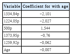
Model 1 using least absolute shrinkage and selection operator

Table 3.

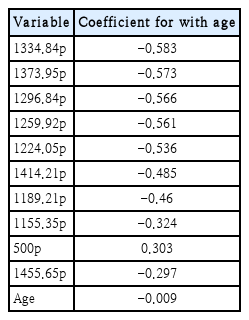
Model 1 using elastic net

Fig. 2.

ROC curves of machine learning results using LASSO or elastic net between normal and chronic otitis media. A: ROC curve for train set from results using LASSO. B: ROC curve for test set from results using LASSO. C: ROC curve for train set from results using elastic net. D: ROC curve for test set from results using elastic net. ROC, receiver operating characteristic; AUC, area under the ROC curve; LASSO, least absolute shrinkage and selection operator.

Model 2의 경우 elastic net을 이용한 방식은 machine learning 중 함수를 도출해내지 못했고, LASSO 방식을 취한 경우 AUC 결과값이 test set에서 0.589로 값이 크지 않았다. Model 2의 경우에는 train set에서 ETD가 6명로 너무 작아서, LASSO에서는 겨우 모형이 추정되었으나 좀 더 복잡한 방법인 Elastic Net에서 회귀모형 추정이 되지 않은 것으로 생각된다.

Model 3의 경우에도 각각 LASSO와 elastic net을 이용한 함수 도출을 진행하였으나 AUC 값이 test set에서 각각 0.601 (LASSO), 0.596 (elastic net)으로 값이 크지 않았다.

본 연구에서는 각 Model 1, 2, 3별로 random forest 분석 또한 진행하였다. Fig. 3은 Model 1의 radom forest machine learning 결과를 나타내고 있으며, Fig. 3A의 그래프는 가장 중요도가 높은 순으로 30개 정도의 변수들을 나열한 것이다. accuracy 값과 Gini 값을 보았을 때, 중요도가 높은 변수로는 1200-1400 Hz 사이의 peak pressure에서의 absorbance와 resonance frequency가 있음을 알 수 있다. Model 1의 경우, random forest 분석 결과의 AUC값이 train set 0.732, test set 0.726로 0.8에 가까웠다(Fig. 3B and C). 반면 Model 2, 3의 경우 test set에서의 AUC값이 각각 0.644, 0.540로 크지 않았다.

Fig. 3.

Random forest analysis in machine learning between normal and chronic otitis media. A: Variables are plotted by the importance. The power of importance of each variable was measured by mean decrease accuracy and mean decrease gini. For variables, the number means frequency, and x or y means whether it is the absorbance at peak pressure or at ambient pressure. Random forest analysis included the variables of age, resonance frequency, peak pressure, and absorbance at peak pressure or at ambient pressure, but variables that measured to have the 30 largest importance were only plotted. B: ROC curve for train set in Model 1 which used machine learning method of random forest. C: ROC curve for test set in Model 1 which used machine learning method of random forest. x: absorbance of frequency at peak pressure. y: absorbance of frequency at ambient pressure. AUC, area under the ROC curve; ROC, receiver operating characteristic.

고 찰

본 연구는 WBT의 결과 변수들을 정상군과 만성중이염군, 이경화증군, 이관개방증군에서 machine learning을 통한 비교 분석으로, resonance frequency, peak pressure, 그리고 ambient pressure에서의 주파수별 absorbance, peak pressure에서의 주파수별 absorbance가 이러한 질환들의 진단에 얼마나 의미가 있는지를 알아보았다. 또한 machine learning을 통하여 그러한 구분을 위한 모델링을 해보았다. 본 연구에서 machine learning을 통한 WBT의 유의미한 구분은 정상군과 만성중이염군에서만 나타났다. 이경화증군과 이관개방증군의 경우 적은 증례로 인하여 유의미한 결과를 얻지 못하였다. 만성중이염군은 정상군에 비하여 resonance frequency 값과 peak pressure 값이 유의미하게 낮았고, LASSO, elastic net을 이용한 machine learning을 통해 구해본 함수에서는 주로 1000-1400 Hz대, 그리고 500 Hz의 peak pressure에서의 absorbance 수치가 두 군의 구분에 중요한 역할을 하였다. 또한 random forest 방식의 machine learning을 통해서는 1200-1400 Hz 사이의 peak pressure에서의 absorbance와 resonance frequency가 두 군의 구분에 중요한 역할을 함을 알 수 있었다.

WBT는 기존의 주로 226 Hz에서의 pressure별 absorbance를 측정하는 tympanometry의 한계를 극복하고자 개발된 방식으로 국내에서는 2017년 우리나라 인구집단에서의 WBT 정상치 및 연령대별 비교를 정리한 바 있으며, 정상, 고막 유착, 고막 천공, 삼출성중이염에서의 WBT 결과를 비교한 바 있다[22,23]. 그 결과로 고막 함입(retration)에서는 2000 Hz 미만에서, 삼출성중이염에서는 500 Hz 이상 모든 주파수에서 정상과 유의한 차이가 있었고, 고막 천공에서는 400 Hz 이하의 저주파에서 정상보다 유의하게 absorbance가 높았으며 1600, 3150 Hz에서는 정상보다 낮았다[22]. 이경화증에서 시행한 WBT에 관한 논문들은[5,13,24-26] WBT의 absorbance 평균값이 250-2000 Hz 사이에서 정상군보다 낮고, resonance frequency는 더 높으며, 1000 Hz에서의 absorbance 값이 정상과의 구분에 있어 가장 민감도와 특이도가 높다는 보고가 있다[13,26]. 한편, 4000-8000 Hz 사이의 평균 absorbance가 이경화증에서 정상보다 더 높다는 보고도 있었고[25], peak pressure에서의 absorbance가 이경화증과 정상을 구분하는 데 유의미하다는 결과도 보고된 바 있었다[5].

이외에도 bone cement를 이용한 이소골 성형술을 시행한 경우와 type I 고실성형술을 시행한 경우, 그리고 정상인 경우를 WBT로 분석, 비교해본 연구가 있었고[27], 이관기능저하 환자들에서 WBT를 시행한 연구가 있다[28]. 이관기능저하 환자들에서 WBT를 시행한 연구의 경우, peak pressure에서의 WBT 데이터와 absolute pressure에서의 WBT 데이터의 차이가 정상에 비해 유의미하게 더 크다는 결론이 제시된 바 있다.

본 연구에서는 중이질환에서의 WBT 데이터에 대한 분석을 machine learning을 통해 시행하고자 하였으며, 이를 통해 WBT 데이터에서 질환 별로 유심히 보아야 할 부분을 찾아보고자 하였다. 본 연구에서는 적은 숫자로 인해 이경화증 환자들에서 machine learning으로 유의미한 차이를 가지는 결과를 찾을 수 없었으나 평균화된 그래프의 전체적인 모습으로 보았을 때는 이전의 연구결과와 비슷하게 1000 Hz에서 2000 Hz 사이의 absorbance 값이 정상에 비해 감소되어 있는 특징을 볼 수 있었다. 이관 개방증의 경우에도 정상군과 유의미하게 구분할 만한 WBT 데이터의 차이는 없었다. 반면 만성중이염의 경우에는 유의미한 차이가 여러 WBT 데이터에서 많이 나타났고, 이러한 결과를 machine learning을 이용하여 분석, 구분할 수 있는 Model을 제작할 수 있었다.

본 연구의 한계점으로는 본 연구의 대상자수가 너무 적었다는 점이 있겠다. 특히나 이경화증군이나 이관개방증군의 경우에는 정상군이 179명인 것에 비해 각각 14명, 24명으로 그 대상자 수가 상당히 적었다. 이러한 결과가 machine learning을 시행한 결과를 분석하는데 상당한 장애가 되었을 것임은 분명하다. 또한 만성중이염군의 경우에는 그 원인이 고막천공부터 이소골문제, 유양동 문제 등 더 분류해볼 수 있는 원인이 많다는 점에서 한계가 있겠다. 향후 이경화증과 이관개방증 환자들을 더 모집하여 추가적인 machine learning을 시행해보는 것이 필요할 것으로 보이며, 만성중이염 환자들의 경우에도 소리전달 경로에 있어서 문제가 되는 부분들별로 나누어 다시 machine learning을 시행해 보는 것도 향후의 연구과제로 남아있다. 아울러 WBT는 데이터의 해석에 있어 parameter와 분석 방법이 다양하여 주의를 하여야 한다는 점에서 한계가 있을 수 있겠다[29,30]. 또한, 비록 Model들을 통해 특정 주파수에서의 차이가 질환들 별로 나타남은 알아낼 수 있었으나, 가장 이상적인 cut off value를 설정하고 그에 따른 train, test set에서의 진단적 유용성을 분석해보지는 못하였다. 그리고 특정 주파수에서의 차이에 대한 임상적 의미나, 이를 해석할 만한 내용 또한 아직 찾지 못했다. 이러한 점 또한 추후 추가적으로 연구되어 봐야할 부분일 것으로 보인다.

결국 이번 연구에서는 WBT로 중이 질환을 진단하는 모델을 제시하지는 못했지만, 본 연구는 WBT 데이터 값의 분석에 machine learning 기법을 도입했다는 점에서 상당한 의의가 있겠다. 금번의 연구에서 볼 수 있듯 WBT 데이터의 경우 자료수가 적고, 그에 비해 변수 개수는 너무 많아서 예측 모형의 과적합(overfit) 문제를 줄이는 통계기법을 사용할 필요가 있다. 그러한 통계기법으로 본 연구에서 사용한 LASSO, elastic net, random forest과 같은 machine learning 기법은 추후에도 WBT 데이터의 분석에 도움이 되리라고 생각된다.

이번 연구에서는 machine learning 방식의 분석을 통해 WBT 결과 중에서도 특정 주파수, 혹은 주파수 범위의 absorbance가 중요한지를 알 수 있었다. 향후 더 많은 대상 수를 이용해 새로 모델링을 해본다면 WBT를 통한 정상군과 이관개방증의 구분이나 정상군과 이경화증의 구분을 위한 모델을 구축하면 WBT 결과값들 중 특정값들만으로 빠르게 진단적 도움을 얻을 수 있으리라고 생각된다.

Article information Continued